Hello there,
Today, we are going to see how to make the first part of our photon mapper. We are unfortunately not going to talk about photons, but only about normal ray tracing.

This is ugly !!! There is no shadow…
It is utterly wanted, shadows will be draw by photon mapping with opposite flux. We will see that in the next article.
Introduction
In this chapter, we are going to see one implementation for a whitted ray tracer
Direct Lighting
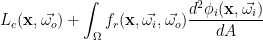
Direct lighting equation could be exprimed by :

The main difficult is to compute the solid angle 
For a simple isotropic spot light, the solid angle could be compute as :

with :
the solid angle.
the total flux carried by the light.
the attenuation get by projected light area on lighted surface area.
- angleCutOff
.
Refraction and reflection
Both are drawn by normal ray tracing.
Architecture
Now, we are going to see how our ray tracer works :
Shapes :
Shapes are bases of renderer. Without any shapes, you can’t have any render. We can have many differents shape, so, we can use one object approach for our shapes.
|
1 2 3 4 5 6 7 8 9 10 11 12 13 14 15 16 17 18 19 20 21 22 23 24 25 26 27 28 29 30 31 32 33 34 35 36 37 38 39 40 |
#ifndef SHAPE_HPP #define SHAPE_HPP #include "ray.hpp" #include "material.hpp" /** * @brief This class provides an interface to manage differents shape */ class AbstractShape { public: AbstractShape() = default; AbstractShape(std::unique_ptr &&material); /** * @brief Return the distance between shape and ray emetter * * @param ray * * @return Negative value if not found. Distance between object and ray emetter */ virtual float intersect(Ray const &ray) const = 0; virtual glm::vec3 getNormal(glm::vec3 const &position) const = 0; /** * @brief Return the radiance returned by the material owned * * @param ray * * @return radiance */ glm::vec3 getReflectedRadiance(Ray const &ray); virtual ~AbstractShape() = default; private: std::unique_ptr mMaterial = std::make_unique(glm::vec3(1.0, 1.0, 1.0), 1.0); }; |
Materials
For each shapes, we obviously have a particular material. The material have to give us a brdf and can reflect radiance.
|
1 2 3 4 5 6 7 8 9 10 11 12 13 14 15 16 17 18 19 20 21 22 23 24 25 26 27 28 29 30 31 32 33 34 35 36 |
/** * @brief This class describes a material */ class AbstractMaterial { public: AbstractMaterial(float albedo); /** * @brief Get the reflected radiance * * @param ray * @param shape Useful to get normal, UV for texture??? * * @return { description_of_the_return_value } */ virtual glm::vec3 getReflectedRadiance(Ray const &ray, AbstractShape const &shape) = 0; virtual void bouncePhoton(Photon const &photon, AbstractShape const &shape) = 0; virtual ~AbstractMaterial() = default; float albedo; protected: /** * @brief Get the Bidirectionnal Reflectance Distribution Function * * @param ingoing * @param outgoing * @param normal * * @return the brdf */ virtual float brdf(glm::vec3 const &ingoing, glm::vec3 const &outgoing, glm::vec3 const &normal) = 0; }; |
Storage Shapes
To have a better ray tracing algorithm, we could use a spatial structure like Kd-tree or other like one :
|
1 2 3 4 5 6 7 8 9 10 11 12 13 14 15 16 17 18 19 20 21 22 23 24 25 |
/** * @brief This class provide a structure to store shapes */ class AbstractShapeStorage { public: /** * @brief Add a shape in structure * * @param shape */ virtual void addShape(std::shared_ptr const &shape) = 0; /** * @brief Get the nearest shape * * @param ray * * @return a tuple with shape and distance. Shape could be null if no shape found */ virtual std::tuple<std::shared_ptr, float> findNearest(Ray const &ray) = 0; ~AbstractShapeStorage() = default; }; |
Algorithm
The main algorithm part is on the materials side. Below, a piece of code where I compute the reflected radiance for a lambertian material and a mirror. You could see that material part has access to other shape via the global variable world.
|
1 2 3 4 5 6 7 8 9 10 11 12 13 14 15 16 17 18 19 20 21 22 23 24 25 26 27 28 29 30 31 |
float LambertianMaterial::brdf(const glm::vec3 &, const glm::vec3 &, glm::vec3 const &) { return albedo / M_PI; } vec3 UniformLambertianMaterial::getReflectedRadiance(Ray const &ray, AbstractShape const &shape) { vec3 directLighting = getIrradianceFromDirectLighting(ray, shape); float f = brdf(vec3(), vec3(), vec3()); return color * f * (directLighting); } float MirrorMaterial::brdf(const vec3&, const vec3&, const vec3&) { return albedo; } vec3 MirrorMaterial::getReflectedRadiance(const Ray &ray, const AbstractShape &shape) { if(ray.recursionDeep >= MAX_BOUNCES) return vec3(); Ray reflectedRay = getReflectedRay(ray, shape.getNormal(ray.origin + ray.direction * ray.distMax)); auto nearest = World::world.findNearest(reflectedRay); if(get(nearest) != nullptr) { reflectedRay.distMax = get(nearest); return brdf(vec3(), vec3(), vec3()) * get(nearest)->getReflectedRadiance(reflectedRay); } return vec3(); } |
Lights
Lighting is a useful feature in a render. It’s thanks to lights that you can see the relief. A light carry a flux. Irradiance is the flux received by a surface.
So, our interface is :
|
1 2 3 4 5 6 7 8 9 10 11 12 13 14 15 16 17 18 19 20 21 22 23 24 25 26 |
/** * @brief Interface for a light */ class AbstractLight { public: AbstractLight(glm::vec3 const &flux); /** * @brief Compute irradiance receive by the projected area in position * * @param position surface's position * @param normal surface's normal * * @return irradiance */ virtual glm::vec3 getIrradiance(glm::vec3 const &position, glm::vec3 const &normal) = 0; virtual void emitPhotons(std::size_t number) = 0; virtual ~AbstractLight() = default; protected: glm::vec3 mTotalFlux; }; |
Below a piece of code about computing irradiance :
|
1 2 3 4 5 6 7 8 9 10 11 12 13 14 |
vec3 SpotLight::getIrradiance(const vec3 &position, const vec3 &normal) { vec3 posToLight = mPosition - position; vec3 posToLightNormalized = normalize(posToLight); if(dot(-posToLightNormalized, mDirection) > mCosCutoff) { float solidAngle = - 2.f * M_PI * (mCosCutoff - 1); return lambertCosineLaw(posToLightNormalized, normal) * mTotalFlux / (solidAngle * dot(posToLight, posToLight)); } return vec3(); } |
The next time, we will see how to integrate a photon mapper to our photon mapper. If you want to have the complete code, you could get it here :
GitHub
Bye my friends :).


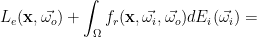
 is the outgoing radiance. It will be our pixel color in R, G, B space. It is exprimed in
  .
. is the emmited radiance. It should be zero for almost all materials, excepting those that emit light (fluorescent material or lights for examples).
 is the Bidirectional Reflectance Distribution Function(aka BRDF). It defines how light is reflected on surface point
  . It is exprimed in
  . Its integral over
  is the incoming radiance. It is like the light received by
  is the lambert cosine law.
 is the differential solid angle. It is exprimed in
  .
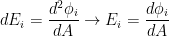
. is differential irradiance. It is the radiant flux (or power) received by a surface per unit area. It is exprimed in
  .
. is the radiant flux(or power) passing from
  . It could be seen as one of our photons. It is exprimed in R, G, B space as well. It is exprimed in
  .
. is the area which received the radiant power.
 .
.
 :
:
 with
with