photon mapping Archives - Page 2 of 2

Introduction:

Hi guys!

I have not written anything here since a long time, I had exams, professional mission in C++ with Qt and too many things to do. Don’t be afraid, activities in this blog will be start again soon.

In computer graphics, I didn’t do beautiful things, except a little ray tracer with photon mapping. I’m going to explain how to make a little photon mapper. Firstly, we’ll see the it on the CPU side, after we’ll try to implement it in the GPU side.

We will see several points :

Explanations about rendering equations
A raytracer
A photon mapper
A GPU side with Photons Volume

Perhaps, some chapters will be divided into several parts.

Rendering Equation :

Rendering_eq

The rendering equation is :

$\displaystyle{L_o(\mathbf{x}, \vec{\omega_o}) = L_e(\mathbf{x}, \vec{\omega_o}) + \int_{\Omega}f_r(\mathbf{x}, \vec{\omega_i}, \vec{\omega_o})L_i(\mathbf{x}, \vec{\omega_i})(\vec{\omega_i}\cdot\vec{n}) d\omega_i =}$
$\displaystyle{L_e(\mathbf{x}, \vec{\omega_o}) + \int_{\Omega}f_r(\mathbf{x}, \vec{\omega_i}, \vec{\omega_o})dE_i(\vec{\omega_i}) =}$
$\displaystyle{L_e(\mathbf{x}, \vec{\omega_o}) + \int_{\Omega}f_r(\mathbf{x}, \vec{\omega_i}, \vec{\omega_o})\frac{d^2 \phi_i(\mathbf{x}, \vec{\omega_i})}{dA}}$

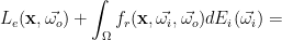
What is it burried into this equation?

$L_o(\mathbf{x}, \vec{\omega_o})$ is the outgoing radiance. It will be our pixel color in R, G, B space. It is exprimed in $W\cdot sr^{-1}\cdot m^{-2}$ .
$L_e(\mathbf{x}, \vec{\omega_o})$ is the emmited radiance. It should be zero for almost all materials, excepting those that emit light (fluorescent material or lights for examples).
$f_r(\mathbf{x}, \vec{\omega_i}, \vec{\omega_o})$ is the Bidirectional Reflectance Distribution Function(aka BRDF). It defines how light is reflected on surface point $\mathbf{x}$ . It is exprimed in $sr^{-1}$ . Its integral over $\Omega$ should be inferior or equal to one.
$L_i(\mathbf{x}, \vec{\omega_i})$ is the incoming radiance. It is like the light received by $\mathbf{x}$ in a direct or indirect way.
$(\vec{\omega_i}\cdot\vec{n})$ is the lambert cosine law.
$d\omega_i$ is the differential solid angle. It is exprimed in $sr$ .
$dE(\vec{\omega_i})$ is differential irradiance. It is the radiant flux (or power) received by a surface per unit area. It is exprimed in $W\cdot m^{-2}$ .
$\phi_i(\mathbf{x}, \vec{\omega_i})$ is the radiant flux(or power) passing from $\mathbf{x}$ and have for direction $\omega_i$ . It could be seen as one of our photons. It is exprimed in R, G, B space as well. It is exprimed in $W$ .
$dA$ is the area which received the radiant power.

Manipulate rendering equation for an approximation

This part is going to be a bit mathematical with “physical approximation :D”.

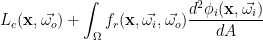
Simplification of irradiance

$\displaystyle{dE_i=\frac{d^2 \phi_i}{dA}\rightarrow E_i=\frac{d\phi_i}{dA}}$

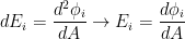
Assuming the “floor” of the hemisphere is flat and photon hitting this floor is like hit $\mathbf{x}$ , we have :

$\displaystyle{E_i \simeq \sum \frac{\phi_i}{\pi r^2}\rightarrow E \simeq \sum_i \sum \frac{\phi_i}{\pi r^2} = \sum \frac{\phi}{\pi r^2}}$ .

So, to have a better approximation, you must have to reduce the hemisphere’s radius and increase the photons number.

The rendering equation simplified

$\displaystyle{L_o(\mathbf{x}, \vec{\omega_o}) = L_e(\mathbf{x}, \vec{\omega_o}) + \int_{\Omega}f_r(\mathbf{x}, \vec{\omega_i}, \vec{\omega_o})L_i(\mathbf{x}, \vec{\omega_i})(\vec{\omega_i}\cdot\vec{n}) d\omega_i =}$
$\displaystyle{L_o(\mathbf{x}, \vec{\omega_o}) = L_e(\mathbf{x}, \vec{\omega_o}) + \frac{1}{\pi r^2}\sum f_r(\mathbf{x}, \vec{\omega_{photon}}, \vec{\omega_o})\phi(\mathbf{x}, \vec{\omega_{photon}})}$

Direct Illumination

Direct illumination need an accurate quality, so, we will not use the simplified equation seen above but the real one. The main difficulty is to compute the solid angle. For example, a point light with power $\phi_L$ :

$\displaystyle{L_r = f_r(\mathbf{x}, \vec{\omega_i},\vec{\omega_o})(\vec{\omega_i}\cdot\vec{n})\frac{\phi_l}{4\pi r^2}}$

We remind that $E = \frac{I}{r^2} = \frac{\phi_l}{\Omega r^2}$ with $\Omega$ the solid angle.

Photon tracing, reflection and refractions

The photon tracing is easy. Imagine you have a 1000W lamp, and you want to share all of its power into 1 000 photons, each photon should have a 1W power (We could say the colour of this photon is (1.0, 1.0, 1.0) in RGB normalized space). When photon hit a surface, you store it into the photon maps and reflect it with the BRDF :).

If you didn’t get it all, don’t be afraid, in our futur implementation, we are going to see how it works. We will probably not do any optimization, but it should be good :).

Bye my friends 🙂 !

CPP Rendering

Tag Archives: photon mapping

How to make a Photon Mapper : Rendering Equation Debunked